ROC Analysis Tool Based on DeLong's Method

Background

Originated from problems of radar and sonar detection in early 1950s, receiver operating characteristic (ROC) analysis has become an indispensable tool to tackle the so-called two-sample problems in many scientific and engineering fields, such as describing the performances of diagnostic systems in clinical medicine, characterizing the overall accuracies of classifiers in machine learning, quantifying the extent of signal detectability in signal processing, and so forth.

In essence, ROC analysis is a supervised research framework that requires prior knowledge of both the sample membership and underlying cumulative distribution functions (cdfs) generating the two samples. Given such knowledge, the procedure of ROC analysis might be initiated from plotting a two-dimensional ROC curve, which is traced out by pairs of false-positive rate and true-positive rate according to various decision threshold settings. With the ROC curve, the area under the curve (AUC) can then be computed, either analytically or empirically, as a figure of merit that might be better than accuracy when characterizing a classifier’s performance.

As revealed by Bamber, AUC can be estimated by the Mann-Whitney U statistic (MWUS). Based on such relationship, a plenty of nonparametric methods have been proposed in the literature. Among algorithms for comparing the areas under two or more correlated receiver operating characteristic (ROC) curves, DeLong’s algorithm is perhaps the most widely used one due to its simplicity of implementation in practice. Recently, we have reduced the time complexity of DeLong’s algorithm from quadratic down to linearithmic order, based on an equivalent relationship between the Heaviside function and mid-ranks of samples.

In this post, I will release the source codes for the two algorithms mentioned in our paper, followed by a brief introduction to a ROC analysis tool published on my GitHub page.

Soure codes

Algorithm 1: Procedure of Calculating Mid-ranks

As our method is based on the relationship between the Heaviside function and mid-ranks of samples, the first step is to calculate the mid-ranks. Presented below is a MATLAB function to achieve this. The input to this function, x, is a 1 by N vector, and the output, T, contains the corresponding mid-ranks.

function T = midrank(x)
%MIDRANK
[Z J] = sort(x);
Z = [Z Z(end) + 1];
N = length(x);
T = zeros(1, N);
i = 1;
while i <= N
    a = i;
    j = a;
    while Z(j) == Z(a)
        j = j + 1;
    end
        b = j - 1;
    for k = a : b
        T(k) = (a + b) / 2;
    end
    i = b + 1;
end
T(J) = T;
end

Algorithm 2: Improved DeLong’s Algorithm

With the midrank function, we can now implement the fast version of DeLong’s algorithm, shown below. The input argument, samples, is a MATLAB struct consisting of two elements:

• spsizes is a 2 x 1 vector, which represents the sizes of two samples, namely, X and Y. For ease of later reference, let m, n denote these two values.
• ratings is a K x N matrix, where each row represents the ratings of one experiments. Note that N must be equal to the sum of m and n, and its first m elements is the ratings corresponding to X, while the last n elements corresponding to Y.

There are two outputs, aucs denotes the AUCs corresponding to each row of the ratings, while delongcov is the covariance matrix.

function [aucs, delongcov] = fastDeLong(samples)
%FASTDELONGCOV
%The fast version of DeLong's method for computing the covariance of 
%unadjusted AUC.
%% [aucs, delongcov] = fastDeLong(samples)
%% 

if sum(samples.spsizes) ~= size(samples.ratings, 2) || numel(samples.spsizes) ~= 2
    error('Argument mismatch error');
end

z = samples.ratings;
m = samples.spsizes(1);
n = samples.spsizes(2);
x = z(:, 1 : m);
y = z(:, m + 1 : end);
k = size(z, 1);

tx = zeros(k, m);
ty = zeros(k, n);
tz = zeros(k, m + n);

for r = 1 : k
    tx(r, :) = midrank(x(r, :));
    ty(r, :) = midrank(y(r, :));
    tz(r, :) = midrank(z(r, :));
end

aucs = sum(tz(:, 1 : m), 2) / m / n - (m + 1) / 2 / n;

v01 = (tz(:, 1 : m) - tx(:, :)) / n;
v10 = 1 - (tz(:, m + 1 : end) - ty(:, :)) / m;

sx = cov(v01')';
sy = cov(v10')';

delongcov = sx / m + sy / n;

end

Introduction of the ROC analysis tool

Furthur more, I have published a UI tool for ROC analysis in my Github page, you can download the sourse codes here.

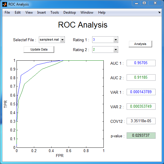
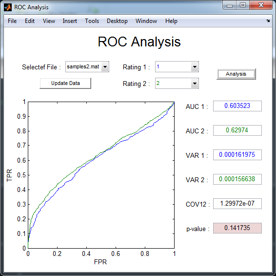
To analyze your own data, you should first move your experiment results, saved as a .mat file in the required format, into the same directory as the source code for this tool. Then run the DeLongUserInterface function, and you will see your file listed in the “Selected File” popup menu. Next, select your file and click the “Update Data” button below - several ROC curves will be drawn based on your data. Now choose the two ratings you would like to analyze under “Rating 1” and “Rating 2”, and click the “Analysis” button. Finally, you will obtain the statistical results. Note that all results are calculated using DeLong’s formulas, implemented efficiently as described by Sun and Xu.

If the text color of a push button is red, it indicates that the results shown in the interface are inconsistent with the options chosen in the popup menu. To fix this, simply click on the corresponding button again. The text color will turn back to black, indicating that the results now match your selected options. This provides a quick visual check to ensure the analysis reflects your choices.

The variables saved in the .mat file are spsizes and ratings, whose meanings have been mentioned in the subsection Algorithm 2.

Citation Request

Anyway, I hope that this tool could be helpful for researchers who using AUC in their work.

If you publish material based on these codes, then, please refer to our paper:

X. Sun, W. Xu, Fast implementation of DeLong's algorithm for comparing the areas under correlated receiver operating characteristic curves, IEEE Signal Processing Letters 21 (11) (2014) 1389-1393.

Here is a BiBTeX citation as well:

@article{sun2014fast,
  title={Fast Implementation of DeLong's Algorithm for Comparing the Areas Under Correlated Receiver Operating Characteristic Curves},
  author={Xu Sun and Weichao Xu},
  journal={IEEE Signal Processing Letters},
  volume={21},
  number={11},
  pages={1389-1393},
  year={2014},
  publisher={IEEE}
}